The numbers that contain everything

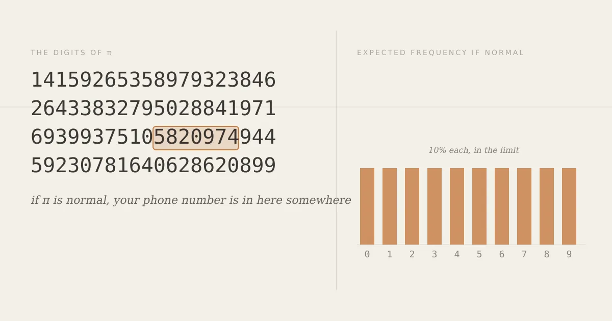
You’ve probably heard the claim that somewhere in the digits of $\pi$ is your phone number. Your birthday too, and, if you encode text as digits, every book ever written.

That claim is often presented as a fact about $\pi$, but it isn’t one. We don’t actually know whether $\pi$ has the property needed to make it true.

The property is called normality. Roughly speaking, a number is normal in base 10 if its digits behave the way we’d expect random digits to behave in the long run: each digit occurs with frequency $1/10$, each two-digit string with frequency $1/100$, each three-digit string with frequency $1/1000$, and so on.

That last part matters. If every finite string occurs with the expected frequency, then every finite string occurs infinitely many times. So a normal number really would contain your phone number, your birthday, and any finite piece of text you care to encode.

What makes normal numbers interesting is the mismatch between what we know in general and what we can prove in particular. Almost every real number is normal. But for familiar constants such as $\pi$, $e$, and $\sqrt{2}$, normality is still unproved.

Making “normal” precise

Saying that the digits of a number “look random” is vague, so let’s make it precise.

Fix a base $b \ge 2$, and write a number $x \in [0,1)$ in base $b$ as

where each digit $d_i$ belongs to $\{0,1,\dots,b-1\}$.

The first thing we might ask is whether each individual digit occurs equally often.

In decimal, that means the proportion of each digit $0,1,\dots,9$ tends to $10\%$.

But this isn’t enough. A sequence could contain the right number of zeroes and ones while arranging them in a very non-random way. Knowing how often individual digits occur tells us nothing about how often blocks such as $00$, $01$, or $314159$ occur.

That leads to the stronger definition.

So in decimal, each digit has frequency $1/10$, each two-digit block has frequency $1/100$, each three-digit block has frequency $1/1000$, and so on.

This is the property behind the claim from the introduction. If a number is normal, then every finite string of digits occurs not merely once, but infinitely many times.

Multiplying $x$ by $b$ shifts its base-$b$ digits one place to the left, and taking the result mod $1$ discards whatever fell off the front – so $b^n x \bmod 1$ has digit sequence $d_{n+1}, d_{n+2}, \dots$. Equidistribution of that sequence on $[0,1)$ is exactly the statement that every digit block appears with its expected frequency. In short, $x$ is normal in base $b$ exactly when $(b^n x \bmod 1)_{n \ge 0}$ is equidistributed on $[0,1)$¹.

Finally, normality depends on the base.

Thus absolutely normal $\implies$ normal in base $b$ $\implies$ simply normal in base $b$, and neither implication can be reversed in general.

There is one important relation between bases. If $b$ and $c$ are multiplicatively dependent – meaning

for some positive integers $m$ and $n$ – then normality in one base is equivalent to normality in the other². So, for example, being normal in base $2$ is equivalent to being normal in base $4$ or base $8$.

For multiplicatively independent bases, no such implication holds: there are numbers normal in one base but not in the other³.

A small technical point: we defined normality for numbers in $[0,1)$, while $\pi = 3.14159\dots$ clearly is not.

This does not matter. The integer part contributes only finitely many digits, and finitely many digits cannot change a limiting frequency. Asking whether $\pi$ is normal is therefore the same as asking whether $0.14159265\dots$ is normal.

More generally, when talking about normality, we can ignore the integer part and look only at the digits after the radix point.

Borel’s theorem: almost all numbers are normal

In 1909, Émile Borel⁴ proved that almost every real number is absolutely normal – normal in every integer base at once.

Here, “almost every” has a precise meaning. The exceptions form a set of Lebesgue measure zero. Equivalently, if $x$ is chosen uniformly at random from $[0,1)$, then $x$ is absolutely normal with probability $1$.

What follows is a modern probabilistic proof, not Borel’s original 1909 argument, but it establishes the same theorem. The basic idea is simple: treat the digits of a randomly chosen number as independent random variables, apply the strong law of large numbers, and then use the fact that there are only countably many bases and finite digit strings to check.

The digits of a random number behave like independent rolls. Fix a base $b$ and choose $x$ uniformly from $[0,1)$. Write

in base $b$.

Suppose we ask for the first three decimal digits to be $3$, $1$, $4$. The numbers with that prefix are exactly those in

an interval of length $0.001 = 10^{-3}$. Since $x$ is uniform on $[0,1)$, the probability of landing in that interval – that is, $P(d_1d_2d_3 = 314)$ – is exactly $10^{-3}$, the same number you’d get from three independent, uniform digit draws: $(1/10)^3$.

Nothing about $314$ was special. Prescribing any $k$ digits $a_1 \dots a_k$ pins $x$ to an interval of length $b^{-k}$, so

The joint probability factors exactly as it should for independent variables – knowing the earlier digits tells you nothing about the next one. The same counting argument works for digits at any $k$ positions, not just a prefix. Each fixed digit cuts the surviving set of $x$’s by a factor of $1/b$, regardless of what the unfixed digits in between are free to do. So fixing $d_{i_1}, \dots, d_{i_k}$ restricts $x$ to a union of intervals of total length $b^{-k}$, giving the same factorization. Apart from the usual ambiguity at numbers with two base-$b$ expansions (like $0.4999\dots = 0.5000\dots$ in base 10 – a countable, hence measure-zero, set of exceptions), the digits

are independent and uniformly distributed over $\{0,1,\dots,b-1\}$.

Now fix one block. Let $s$ be some string of $k$ digits. We want to know how often $s$ appears in the expansion of $x$.

There’s a small complication, though: consecutive occurrences can overlap. Take $k=3$ and $s = 314$: the block starting at position $1$ uses $d_1d_2d_3$, while the block starting at position $2$ uses $d_2d_3d_4$ – they share two digits, so the corresponding events aren’t independent, and the law of large numbers doesn’t directly apply.

Split the starting positions into $k$ groups by residue modulo $k$. For $k=3$, that’s $1,4,7,10,\dots$, then $2,5,8,11,\dots$, then $3,6,9,12,\dots$. Within the first group, the blocks $d_1d_2d_3,\ d_4d_5d_6,\ d_7d_8d_9,\dots$ use completely disjoint digits, so they’re independent – each equal to $314$ with probability $1/1000$. The strong law of large numbers says the fraction of these blocks equal to $314$ converges to $1/1000$ almost surely, and the same holds for the other two groups. Since the three groups split the starting positions evenly, their combined frequency is still $1/1000$.

The same argument applies for a block of any length $k$: split the starting positions into $k$ groups by residue modulo $k$, apply the strong law within each group – where the blocks are disjoint and hence independent, each equal to $s$ with probability $1/b^k$ – and recombine. That gives

almost surely, where $n$ counts starting positions rather than digits used (counting only blocks that fit entirely within the first $n$ digits, via $i \le n-k+1$, gives the same limit). For any fixed base $b$, block length $k$, and block $s$, the set of numbers for which the required frequency fails has measure zero.

There are only countably many conditions. Normality asks for this statement to hold for every finite block, and absolute normality asks for it to hold in every integer base.

But there are only countably many choices involved: countably many bases $b\ge2$, countably many lengths $k\ge1$, and finitely many strings of each fixed length in each base. Altogether, there are still only countably many conditions.

Each condition has a measure-zero exceptional set. A countable union of measure-zero sets still has measure zero.

Outside that union, every finite block has the expected limiting frequency in every base. In other words, almost every real number is absolutely normal.

That is Borel’s theorem.

The catch: we can’t prove it for the numbers we care about

Borel’s theorem tells us that almost every real number is normal, and in fact absolutely normal. But take the numbers that turn up naturally in mathematics – $\pi$, $e$, $\sqrt{2}$ – and the situation is very different.

We do not know whether any of them is normal in base 10. In base 2, we cannot even prove the weaker statement that their zeroes and ones occur equally often⁵.

Explicit normal numbers are known – if we are allowed to build a number specifically for the purpose. The simplest is Champernowne’s constant⁶,

formed by writing the positive integers one after another. Champernowne proved in 1933 that this number is normal in base 10. Explicit absolutely normal numbers are also known⁷.

And it is easy to write down numbers that are not normal. Every rational number has an eventually periodic expansion in any integer base; a periodic expansion can only ever realize a bounded number of distinct length-$k$ blocks, while there are $b^k$ possible ones, so most blocks of that length never occur at all, which rules out normality. The usual Liouville constant,

is another example in base 10. Its $1$’s become increasingly sparse – the proportion of $1$’s among the first $n$ digits tends to $0$, not $1/10$ – so even the individual digits fail to occur with equal limiting frequency.

The standard Liouville constant above is not normal, but being a Liouville number does not itself prevent normality: there are Liouville numbers that are normal, as well as ones that are normal in no base⁸. It is the particular digit structure of the constant above, not its membership in the Liouville numbers as a class, that makes it non-normal.

For $\pi$, computation gives us plenty of evidence but no proof. In 2016, Peter Trueb analyzed the first 22,459,157,718,361 decimal digits of $\pi$ and, separately, the first 18,651,926,753,033 hexadecimal digits⁹, counting every block of length one, two, and three in each expansion. The observed frequencies were consistent with what normality predicts. But any finite computation can only examine a finite prefix. Normality is a statement about what happens as the number of digits tends to infinity, so no amount of checking alone can settle it.

We can compute the digits of $\pi$ and $e$ to enormous precision, prove that both are transcendental, and write down series, products, integrals, and rapidly converging algorithms for calculating them. None of those descriptions has yielded the digit-frequency estimates needed to prove normality.

The equidistribution formulation from earlier makes the difficulty concrete. To prove that $\pi$ is normal in base $b$, we would need to show that

is equidistributed in $[0,1)$. This isn’t a matter of computing more digits. It’s about understanding the long-term behavior of the fractional parts of $b^n\pi$ for arbitrarily large $n$. The familiar representations of $\pi$ – geometric and analytic – have not yielded a proof of the required equidistribution.

Why “almost every” tells us so little about one number

There is no contradiction between saying that almost every real number is normal and admitting that we cannot prove normality for $\pi$.

A set of measure zero does not have to be empty, or even small in any ordinary sense. It can be infinite and highly structured. Measure tells us how large a set is inside the continuum of real numbers; it does not tell us whether a particular number belongs to it.

The same gap shows up with transcendence. Almost every real number is transcendental. The algebraic numbers are countable, so they have measure zero. But this fact alone tells us nothing about whether a specific number is transcendental.

Proving that $e$ is transcendental required Hermite’s work in 1873¹⁰. Lindemann proved the transcendence of $\pi$ in 1882¹¹. And even today, we do not know whether a number as simple to write down as

is transcendental¹². In fact even the weaker question, whether $\pi + e$ is irrational, is open.

The theorem that almost every number is transcendental does not help with that question. It says that a randomly chosen real number will avoid the exceptional set with probability $1$. $\pi + e$ is one particular point, and a measure-theoretic statement about almost all points does not tell us where that point lies.

Borel’s theorem has the same limitation. It tells us that the non-normal numbers occupy a measure-zero part of the real line. It does not give us a test that we can apply to $\pi$, $e$, or $\sqrt{2}$.

“Almost every number is normal” tells us a great deal about the real numbers as a whole, and almost nothing about any particular number we happen to care about.

So, does $\pi$ contain your phone number?

We don’t know.

If $\pi$ is normal, then yes: your phone number appears somewhere in its decimal expansion, and not just once, but infinitely many times. The same would be true of your birthday, this article encoded as digits, and every other finite string.

Borel’s theorem tells us that this is what happens for almost every real number. Computations tell us that the digits of $\pi$ behave as normality would predict, in the tests performed so far.

The claim behind the phone-number story – that $\pi$ contains every finite sequence of digits – is still unproved, no matter how plausible it looks.

Borel’s theorem is more than a century old. The simplest questions it raises about specific numbers are still open: is $\pi$ normal? Is $e$ normal? Is $\sqrt{2}$ normal? All three are widely believed to be normal, but nobody has found a way to prove it.