What is π, really?

Most of us meet $\pi$ as the ratio of a circle’s circumference to its diameter. It is a clean definition, easy to state and easy to remember. But it does not explain why the same number shows up in probability, infinite sums, and even problems about counting.

That wider story is what makes $\pi$ so interesting.

The definition you were taught

Take any circle: a coin, a plate, or a planet. Measure its circumference $(C)$ and its diameter $(d)$, then divide one by the other. You will always get the same number: $\pi$, about $3.14159$.

This works because all circles have the same shape. Make a circle twice as wide and its circumference also becomes twice as long, so the ratio stays fixed.

That is a perfectly good definition of $\pi$. The surprise is that it turns up far beyond geometry.

First stop: a stick on the floor

Consider a floor ruled with parallel lines, spaced $t$ apart, and a needle of length $\ell$, where $\ell \leq t$. Drop the needle at random. Sometimes it crosses a line and sometimes it does not. Repeat this thousands of times and count the crossings.

You might expect to learn something about needles and floors. Instead, you can use the results to estimate $\pi$.

If you drop the needle $n$ times and it crosses a line $x$ times, then:

This is Buffon’s needle problem, posed by Georges-Louis Leclerc in 1777. It is one of the earliest examples of a Monte Carlo method, which uses random experiments to estimate a fixed quantity. People have actually recovered several decimal places of $\pi$ by dropping sticks.

Why does $\pi$ appear? The needle lands at an angle $\theta$ relative to the lines, and that angle is uniformly random on $[0,\pi)$. When we account for every possible angle and position, $\pi$ falls out of the geometry of the angle itself.

The probability of a crossing is:

No circle is drawn on the floor. But angles are measured in radians, and radians are built from circle geometry. $\pi$ is already nearby.

Second stop: an infinite sum

In 1644, Pietro Mengoli asked a question that puzzled mathematicians for nearly a century: what is the exact value of this endless sum?

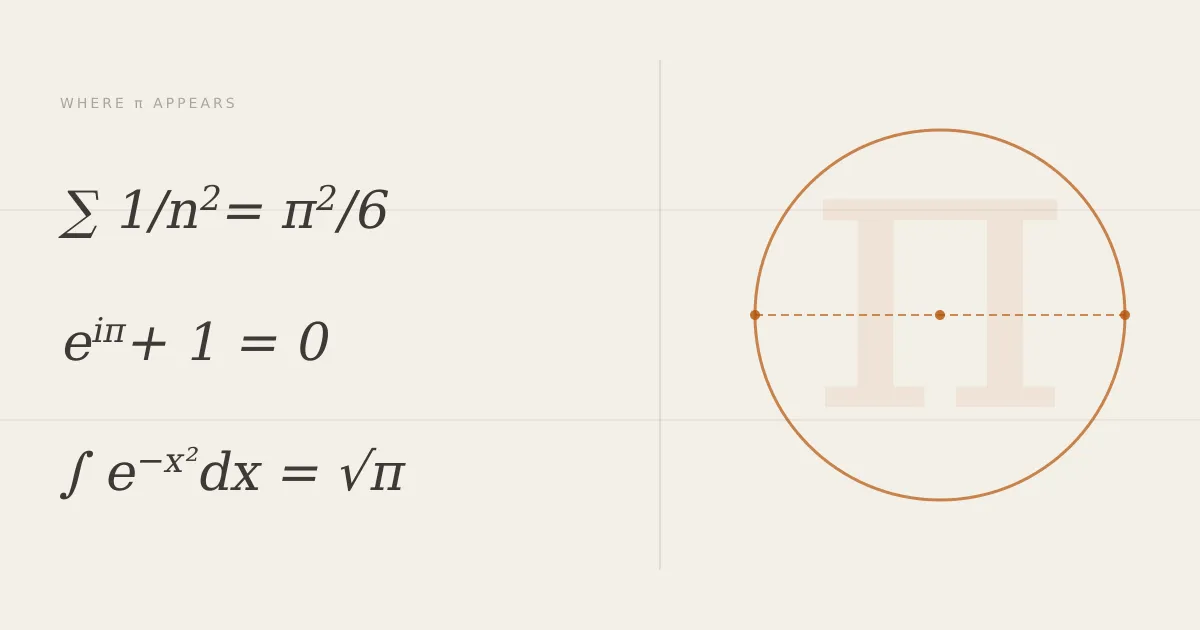
The sum is finite, but for nearly a century nobody could find its exact value. In 1734, Leonhard Euler found the answer:

Why should adding fractions involving square numbers produce $\pi$? The link comes through the sine function. Euler found that $\sin(x)$ can be written as an infinite product:

The important detail is where sine equals zero: $0, \pm\pi, \pm2\pi, \pm3\pi, \ldots$. Expand this product and compare it with the Taylor series for $\sin(x)$, and the coefficient of $x^3$ forces the sum to equal $\pi^2/6$. The regular rhythm of sine carries $\pi$ with it.

3Blue1Brown has a beautiful visual proof of this.

There is an even stranger link to prime numbers. The probability that two randomly chosen integers are coprime, meaning they share no factor other than 1, is $6/\pi^2$, or about 61%. $\pi$ has no obvious business being in number theory, and yet there it is.

Third stop: the bell curve

This is often the most surprising example.

Consider $e^{-x^2}$. It makes a bell-shaped curve, related to the patterns behind measurement errors, heights, and noise in signals. It is one of the central shapes in probability and statistics.

Now integrate it over the entire real line:

$\pi$ is hiding in the area under this curve. Why?

The usual trick is to call the integral $I$, then square it:

Squaring the integral lets us view it over the whole plane. Now switch to polar coordinates, where $x^2+y^2=r^2$ and the area element $dx\,dy$ becomes $r\,dr\,d\theta$. The double integral becomes:

So $I = \sqrt\pi$. The original curve did not mention circles, but the two-dimensional version has circular symmetry. Polar coordinates make that symmetry visible, and $\pi$ comes along with it.

This $\sqrt\pi$ is not an extra detail. In the normal distribution, the familiar bell curve used in statistics, science, and machine learning, $\pi$ appears in the denominator:

The $\sqrt{2\pi}$ makes the total area under the curve equal to 1. Without it, the curve could not represent probabilities.

3Blue1Brown has a visual walkthrough of the polar coordinates argument.

Fourth stop: counting things

Factorials are about counting. For example, $5!$ is the number of ways to arrange five books on a shelf. So it feels odd to find $\pi$ in a formula about factorials.

For large $n$, Stirling’s approximation gives:

The $\sqrt{2\pi n}$ is essential. Without it, the estimate is much less accurate; with it, the relative error shrinks as $n$ grows.

Why is it there? The Gamma function gives an exact integral for a factorial: $n! = \Gamma(n+1) = \int_0^\infty t^n e^{-t} \, dt$. For large $n$, the integrand peaks sharply near $t=n$, and near that peak it is shaped like a Gaussian. Evaluating that Gaussian peak is the same computation as the bell curve integral, so $\pi$ appears for the same reason.

The Gamma function also works beyond positive integers, and it still contains $\pi$: $\Gamma(1/2) = \sqrt\pi$. Counting and continuous mathematics are more connected than they first appear.

Fifth stop: a formula nobody expected

In 1748, Euler published what is now called Euler’s identity:

Five famous constants appear in one equation: $e$, $i$, $\pi$, $1$, and $0$. There are no circles or geometric objects in the setup, only the exponential function and imaginary numbers. So why is $\pi$ involved?

The answer is Euler’s formula:

This formula follows from the power series for $e^z$. Put $ix$ into that series and separate the real and imaginary parts; the familiar series for $\cos x$ and $\sin x$ appear.

Geometrically, an imaginary exponent makes $e^{ix}$ travel around the unit circle. As $x$ increases, it moves at a steady rate and completes one full loop at $x=2\pi$.

Try dragging the point around the circle below. The blue value is the real part, $\cos\theta$, and the green value is the imaginary part, $\sin\theta$.

Set $x = \pi$. Since $\cos\pi = -1$ and $\sin\pi = 0$:

And so $e^{i\pi} + 1 = 0$.

$\pi$ appears because $x=\pi$ means a half-turn around the unit circle. This is the same circle geometry behind $C/d=\pi$. The formula also explains why $\pi$ keeps returning wherever sines and cosines describe repeating motion: in sound, waves, and quantum mechanics.

So what is π, really?

Imagine mathematicians who discovered calculus before they studied geometry. They could meet $\pi$ through the bell curve, the Basel problem, or the Gamma function. Later, when they finally studied circles, they might be surprised to find the same number waiting there too.

The schoolbook definition is not wrong. It is one view of a much larger idea. Circles are where $\pi$ is easiest to see, but they are not its only home.

$\pi$ is a constant that appears throughout continuous mathematics. You see it in angles, infinite sums, probability, and counting. A circle is one expression of it; Euler’s identity is another.

The ratio $C/d = \pi$ remains a valid definition. But it is also a doorway into a number that connects many parts of mathematics.

Last updated 7 August 2026